40 excel chart labels from cells

Custom Axis Labels and Gridlines in an Excel Chart 23.7.2013 · Select the vertical dummy series and add data labels, as follows. In Excel 2007-2010, go to the Chart Tools > Layout tab > Data Labels > More Data label Options. In Excel 2013, click the “+” icon to the top right of the chart, click the right arrow next to Data Labels, and choose More Options…. How to Change Excel Chart Data Labels to Custom Values? 5.5.2010 · When you “add data labels” to a chart series, excel can show either “category” , ... Col A is x axis labels (hard coded, no spaces in strings, text format), with null cells in between. The labels are every 4 or 5 rows apart with null in between, marking month ends, the data columns are readings taken each week.

How to Add Labels to Scatterplot Points in Excel - Statology Next, highlight the cells in the range B2:C9. Then, click the Insert tab along the top ribbon and click the Insert Scatter (X,Y) option in the Charts group. The following scatterplot will appear: Step 3: Add Labels to Points. Next, click anywhere on the chart until a green plus (+) sign appears in the top right corner.

Excel chart labels from cells

How to link a cell to chart title/text box in Excel? 3. Go to the formula bar, and type the equal sign = into the formula bar, then select the cell you want to link to the chart title. See screenshot: 4. Press Enter key. Then you can see the selected cell is linked to chart title. Now when the cell A1 changes its contents, the chart title will automatically change. Link a chart title, label, or text box to a worksheet cell On the Format tab, in the Current Selection group, click the arrow next to the Chart Elements box, and then click the chart element that you want to use. In the formula bar, type an equal sign ( = ). In the worksheet, select the cell that contains the data that you want to display in the title, label, or text box on the chart. How to Use Cell Values for Excel Chart Labels 12.3.2020 · Uncheck the “Value” box and check the “Value From Cells” box. Select cells C2:C6 to use for the data label range and then click the “OK” button. The values from these cells are now used for the chart data labels. If these cell values change, then the chart labels will automatically update. Link a Chart Title to a Cell Value

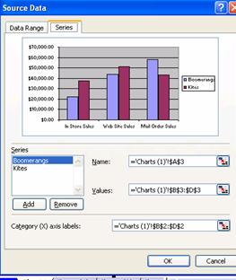
Excel chart labels from cells. How to group (two-level) axis labels in a chart in Excel? The Pivot Chart tool is so powerful that it can help you to create a chart with one kind of labels grouped by another kind of labels in a two-lever axis easily in Excel. You can do as follows: 1. Create a Pivot Chart with selecting the source data, and: (1) In Excel 2007 and 2010, clicking the PivotTable > PivotChart in the Tables group on the ... excel - Stack Overflow Some of the data labels of these charts, get data " From Cells " but this range is still referencing the the first workbook and I need to change it to reference the new sheet in the new workbook. I am being able to get the formula that references the "From Cells". This is the code that I have How to rotate axis labels in chart in Excel? 3. Close the dialog, then you can see the axis labels are rotated. Rotate axis labels in chart of Excel 2013. If you are using Microsoft Excel 2013, you can rotate the axis labels with following steps: 1. Go to the chart and right click its axis labels you will rotate, and select the Format Axis from the context menu. 2. Pivot Chart data labels; value from cells | MrExcel ... I have a pivot chart that shows number of days (vertical axis) by contract (horizontal axis) with a slicer to filter by office. My supervisor wanted me to display the contractor's name on each column. After adding data labels, I stumbled upon the Value from Cells option and when I selected it, the Data Label Range box opened.

The XY Chart Labeler Add-in - AppsPro 1.7.2007 · Delete Chart Labels - Allows you to quickly delete data labels from a single chart series or all series on a chart. Even though this utility is called the XY Chart Labeler, it is capable of labeling any type of Excel chart series that will accept data labels. Download. Windows - Download the XY Chart Labeler for Windows (Version 7.1.07) Automatically set chart axis labels from cell contents The (tick) labels occur at each > major tick along the axis. > > You can link the text of an axis title to a particular cell. Select the > axis title, press the equals key, and select the cell. > > This also works with the chart title, individual data labels, and text > boxes. > > - Jon > ------- > Jon Peltier, Microsoft Excel MVP Add Data Labels From Different Column In An Excel Chart A.docx Manually Add Data Labels From Different Column In An Excel Chart This method will guide you to manually add a data label from a cell of different column at a time in an Excel chart. 1. Right click the data series in the chart, and select Add Data Labels > Add Data Labels from the context menu to add data labels. 2 . Add or remove data labels in a chart - support.microsoft.com Click Label Options and under Label Contains, pick the options you want. Use cell values as data labels You can use cell values as data labels for your chart. Right-click the data series or data label to display more data for, and then click Format Data Labels. Click Label Options and under Label Contains, select the Values From Cells checkbox.

Data Labels Show [CELLRANGE] Rather Than the Expected ... Figure 3: Values from Cells in PowerPoint 2016 This Value From Cells option is a huge improvement over the conventional Value option, and lets you choose a range different than the Values range in the Excel datasheet. To do so, you click the Select Range… button next to the Value From Cells option, shown highlighted in red within Figure 3, above.. As mentioned, clicking the Select Range ... Using the CONCAT function to create custom data labels for ... Check the Value From Cells checkbox and select the cells containing the custom labels, cells C5 to C16 in this example. It is important to select the entire range because the label can move based on the data. Uncheck the Value checkbox because the value is incorporated in our custom label. The dialog box will look like this. › charts › variance-clusteredActual vs Budget or Target Chart in Excel - Variance on ... Aug 19, 2013 · Next you will right click on any of the data labels in the Variance series on the chart (the labels that are currently displaying the variance as a number), and select “Format Data Labels” from the menu. On the right side of the screen you should see the Label Options menu and the first option is “Value From Cells”. › documents › excelHow to wrap X axis labels in a chart in Excel? Some users may want to wrap the labels in the chart axis only, but not wrap the label cells in the source data. Actually, we can replace original labels cells with formulas in Excel. For example, you want to wrap the label of "OrangeBBBB" in the axis, just find out the label cell in the source data, and then replace the original label with the ...

Excel Is Fun

How to add data labels from different column in an Excel ... This method will guide you to manually add a data label from a cell of different column at a time in an Excel chart. 1. Right click the data series in the chart, and select Add Data Labels > Add Data Labels from the context menu to add data labels. 2.

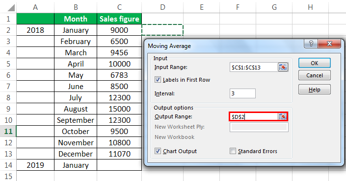
Calculate Moving Average in Excel (Simple, Exponential and Weighted)

Excel Chart Vertical Axis Text Labels • My Online ... So all we need to do is get that bar chart into our line chart, align the labels to the line chart and then hide the bars. We’ll do this with a dummy series: Copy cells G4:H10 (note row 5 is intentionally blank) > CTRL+C to copy the cells > select the chart > CTRL+V to paste the dummy data into the chart.

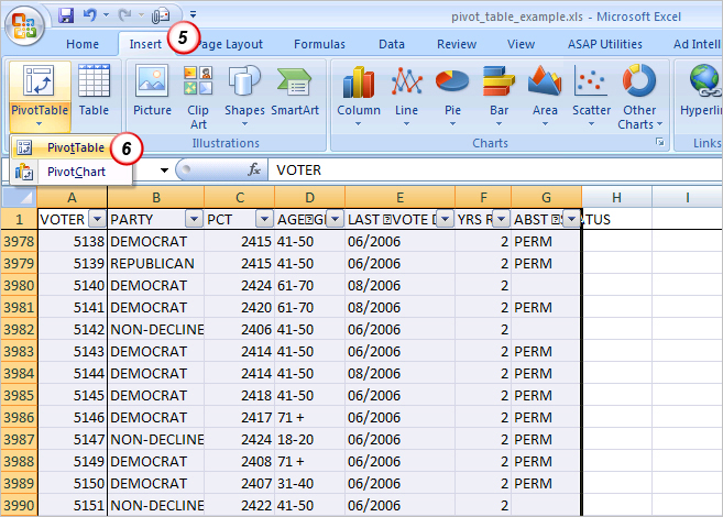
In Search of the Elusive Pivot Table | Dynamic Edge, Inc. | Beyond Tech Support Dynamic Edge ...

chandoo.org › wp › budget-vs-actual-chart-free-templateFree Budget vs. Actual chart Excel Template - Download May 16, 2018 · Step 12: Plug our smart labels in to the chart. Now that we have gorgeous labels, let’s replace the old ones with these. Select first line (budget)’s labels and press CTRL+1 to go to format options. Click on “Value from cells” option and point to Var 1 column. Repeat the process for second line (actual) labels too. We get this.

Share :