42 excel graph data labels different series
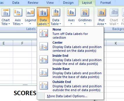
How to Change Excel Chart Data Labels to Custom Values? First add data labels to the chart (Layout Ribbon > Data Labels) Define the new data label values in a bunch of cells, like this: Now, click on any data label. This will select "all" data labels. Now click once again. At this point excel will select only one data label. Go to Formula bar, press = and point to the cell where the data label ... Series.DataLabels method (Excel) | Microsoft Docs Return value. Object. Remarks. If the series has the Show Value option turned on for the data labels, the returned collection can contain up to one label for each point. Data labels can be turned on or off for individual points in the series. If the series is on an area chart and has the Show Label option turned on for the data labels, the returned collection contains only a single label ...
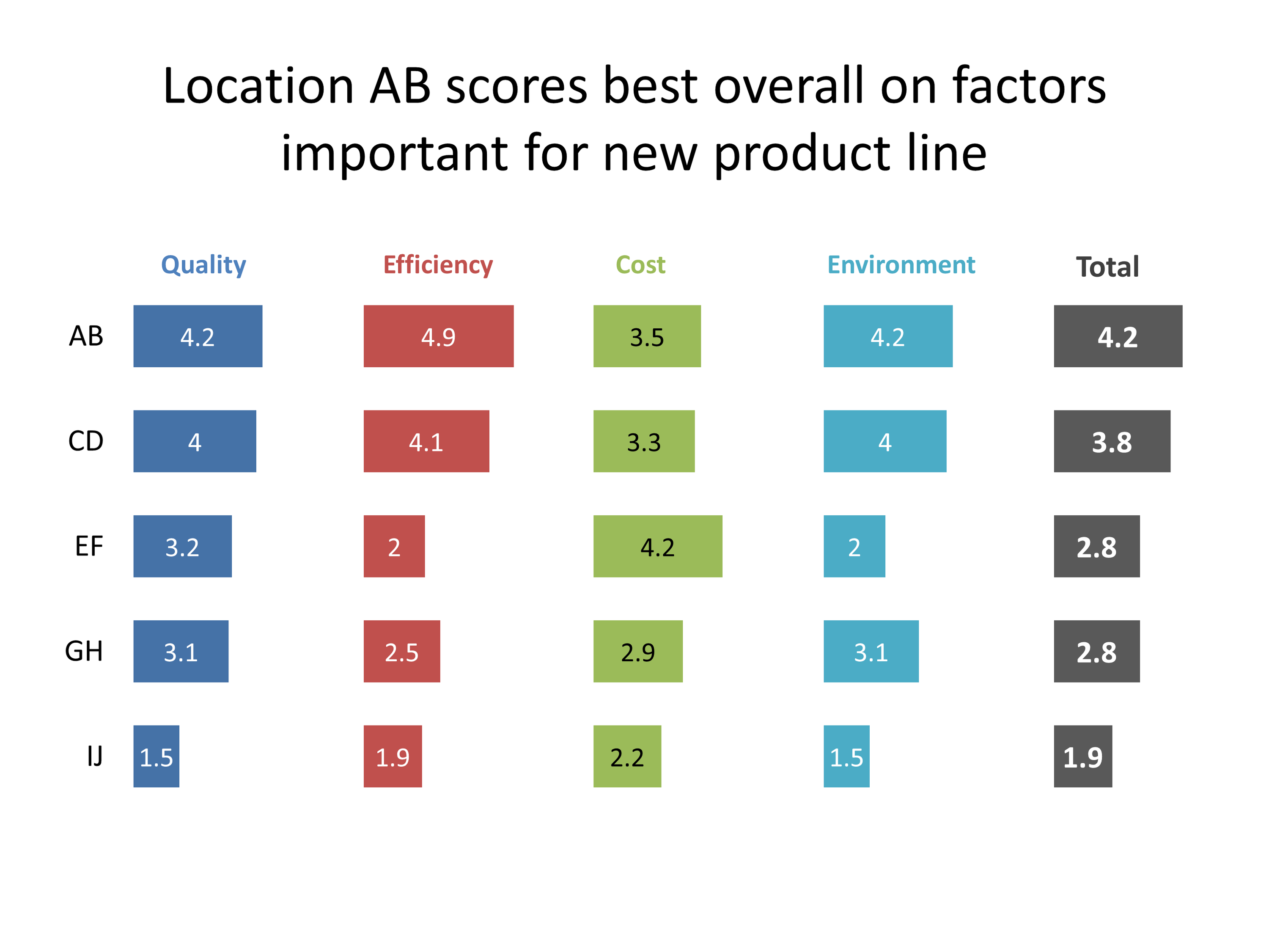
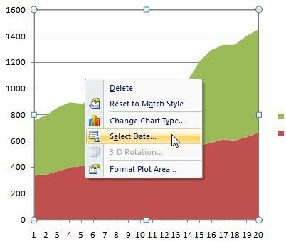
Multiple Series in One Excel Chart - Peltier Tech Select Series Data: Right click the chart and choose Select Data from the pop-up menu, or click Select Data on the ribbon. As before, click Add, and the Edit Series dialog pops up. There are spaces for series name and Y values. Fill in entries for series name and Y values, and the chart shows two series.
Excel graph data labels different series
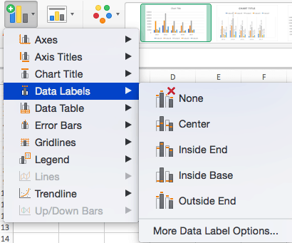
How to Create a Graph with Multiple Lines in Excel Click Select Data button on the Design tab to open the Select Data Source dialog box. Select the series you want to edit, then click Edit to open the Edit Series dialog box. Type the new series label in the Series name: textbox, then click OK. Switch the data rows and columns - Sometimes a different style of chart requires a different layout ... Change the format of data labels in a chart Tip: To switch from custom text back to the pre-built data labels, click Reset Label Text under Label Options. To format data labels, select your chart, and then in the Chart Design tab, click Add Chart Element > Data Labels > More Data Label Options. Click Label Options and under Label Contains, pick the options you want. Vary the colors of same-series data markers in a chart Automatically vary all data marker colors by point or by slice. In a chart, click to select the data series for which you want to change the colors. On the Format tab, in the Current Selection group, click Format Selection. In the Format Data Series pane, click the Fill & Line tab, expand Fill, and then do one of the following:
Excel graph data labels different series. Add a data series to your chart - support.microsoft.com Add a data series to a chart on a chart sheet. On the worksheet, in the cells directly next to or below the source data of the chart, type the new data and labels you want to add. Click the chart sheet (a separate sheet that only contains the chart you want to update). On the Chart Design tab, click Select Data. How to set multiple series labels at once - Microsoft Tech Community Click anywhere in the chart. On the Chart Design tab of the ribbon, in the Data group, click Select Data. Click in the 'Chart data range' box. Select the range containing both the series names and the series values. Click OK. If this doesn't work, press Ctrl+Z to undo the change. Apr 09 2022 12:02 PM. Multiple data labels (in separate locations on chart) Re: Multiple data labels (in separate locations on chart) You can do it in a single chart. Create the chart so it has 2 columns of data. At first only the 1 column of data will be displayed. Move that series to the secondary axis. You can now apply different data labels to each series. Attached Files. excel - Change Multiple Chart Series Labels - Stack Overflow I have around 50 charts each on different sheets. Each chart shows a time series as series one and its trend as series 2 and they are labeled Series 1 and Series 2. ... Excel chart changing all data labels from value to series name simultaneously. 0.
how to add data labels into Excel graphs - storytelling with data There are a few different techniques we could use to create labels that look like this. Option 1: The "brute force" technique. The data labels for the two lines are not, technically, "data labels" at all. A text box was added to this graph, and then the numbers and category labels were simply typed in manually. Dynamically Label Excel Chart Series Lines - My Online Training Hub Step 1: Duplicate the Series. The first trick here is that we have 2 series for each region; one for the line and one for the label, as you can see in the table below: Select columns B:J and insert a line chart (do not include column A). To modify the axis so the Year and Month labels are nested; right-click the chart > Select Data > Edit the ... Excel graphs not identifying Series labels - Microsoft Community Right click the chart in Excel and click 'Select Data'. Make sure that the selection for that graph includes the cells with the names in them. If that still does not automatically name the Series on that dialog, select a series and click 'Edit' which will allow you to edit the Series Name. Change the labels in an Excel data series | TechRepublic Click the Chart Wizard button in the Standard toolbar. Click Next. Click the Series tab. Click the Window Shade button in the Category (X) Axis. Labels box. Select B3:D3 to select the labels in ...
Formating all data labels in a single series at once. Report abuse. Luke Moraga. Xbox Ambassador. Replied on September 21, 2010. When you go to format the data label, make sure the Name Box says you have the whole Data Label collection selected, not just a single data label. Then you can format all of them in 1-shot (either right click and format, or use the Ctrl+1 keyboard shortcut) Data labels using values from different series - Excel Help Forum One way, not elegant but workable, is to add a third data series using the values from the first series as the data and the valus that show the % change as the data labels for the third series. Format the data labels to show the way you want (PHD has some great tips on chart label formatting) Set the third series name to "" and the fill to No ... How to Rename a Data Series in Microsoft Excel To begin renaming your data series, select one from the list and then click the "Edit" button. In the "Edit Series" box, you can begin to rename your data series labels. By default, Excel will use the column or row label, using the cell reference to determine this. Replace the cell reference with a static name of your choice. excel - Change format of all data labels of a single series at once ... A quick way to solve this is to: Go to the chart and left mouse click on the 'data series' you want to edit. Click anywhere in formula bar above. Don't change anything. Click the 'tick icon' just to the left of the formula bar. Go straight back to the same data series and right mouse click, and choose add data labels.
Small Multiples Calculator | Think Outside The Slide
Edit titles or data labels in a chart - support.microsoft.com To edit the contents of a title, click the chart or axis title that you want to change. To edit the contents of a data label, click two times on the data label that you want to change. The first click selects the data labels for the whole data series, and the second click selects the individual data label. Click again to place the title or data ...

How to Import, Graph, and Label Excel Data in MATLAB: 13 Steps
Create a multi-level category chart in Excel - ExtendOffice 2. Select the data range, click Insert > Insert Column or Bar Chart > Clustered Bar.. 3. Drag the chart border to enlarge the chart area. See the below demo. 4. Right click the bar and select Format Data Series from the right-clicking menu to open the Format Data Series pane.. Tips: You can also double click any of the bars to open the Format Data Series pane.

Create a time series plot of multiple Y variables - Minitab Express
How to group (two-level) axis labels in a chart in Excel? Create a Pivot Chart with selecting the source data, and: (1) In Excel 2007 and 2010, clicking the PivotTable > PivotChart in the Tables group on the Insert Tab; (2) In Excel 2013, clicking the Pivot Chart > Pivot Chart in the Charts group on the Insert tab. 2. In the opening dialog box, check the Existing worksheet option, and then select a ...
How to create a chart in excel(18 examples, with add trendline, gridlines, data labels overlap ...
Add or remove data labels in a chart - support.microsoft.com On the Design tab, in the Chart Layouts group, click Add Chart Element, choose Data Labels, and then click None. Click a data label one time to select all data labels in a data series or two times to select just one data label that you want to delete, and then press DELETE. Right-click a data label, and then click Delete.
how to make a excel graph.
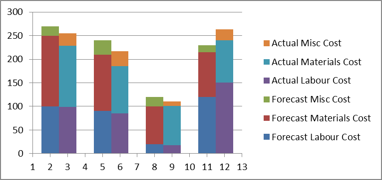
Some Data Labels On Series Are Missing - Excel Help Forum Hi all, Using Excel 2016. I thought I was done with my clustered stacked column chart, so I added Data Labels Inside End - perfect! I then copied the data to some helper cells, filled any missing category labels, sorted the data to show some different grouping on the category axis and pasted the newly rearranged data back to the original cells.

storytelling with data: plotting a value within a range
Format data labels for each series in a chart - Stack Overflow To select a single data point, click on the target series, and then: 1) click again on the target data point, or 2) press the right arrow, to select the first data point. Then to add a data label, right click on the data point, and Add Data Label. Then to select a single data label, click on the data label once (this selects all data labels for ...
How to Make Charts and Graphs in Excel | Smartsheet
How to add data labels from different column in an Excel chart? This method will guide you to manually add a data label from a cell of different column at a time in an Excel chart. 1. Right click the data series in the chart, and select Add Data Labels > Add Data Labels from the context menu to add data labels. 2. Click any data label to select all data labels, and then click the specified data label to ...

Data labels on Excel charts « projectwoman.com
Label line chart series - Get Digital Help To label each line we need a cell range with the same size as the chart source data. Simply copy the chart source data range and paste it to your worksheet, then delete all data. All cells are now empty. Copy categories (Regions in this example) and paste to the last column (2018). Those correspond to the last data points in each series.
How to Change Labels for a Chart Axis in Excel 2007
Vary the colors of same-series data markers in a chart Automatically vary all data marker colors by point or by slice. In a chart, click to select the data series for which you want to change the colors. On the Format tab, in the Current Selection group, click Format Selection. In the Format Data Series pane, click the Fill & Line tab, expand Fill, and then do one of the following:

Creating Graphs in Excel to Support Your Findings in Google Analytics
Change the format of data labels in a chart Tip: To switch from custom text back to the pre-built data labels, click Reset Label Text under Label Options. To format data labels, select your chart, and then in the Chart Design tab, click Add Chart Element > Data Labels > More Data Label Options. Click Label Options and under Label Contains, pick the options you want.

Elements of an Excel Chart | ExcelDemy.com
How to Create a Graph with Multiple Lines in Excel Click Select Data button on the Design tab to open the Select Data Source dialog box. Select the series you want to edit, then click Edit to open the Edit Series dialog box. Type the new series label in the Series name: textbox, then click OK. Switch the data rows and columns - Sometimes a different style of chart requires a different layout ...

| Pryor Learning Solutions
Step-by-step tutorial on creating clustered stacked column bar charts (for free) | Excel Help HQ

Excel Chart Format: How to create dynamic chart labels with Data Label Range and Callout - YouTube

How to Add Data Labels to an Excel 2010 Chart - dummies
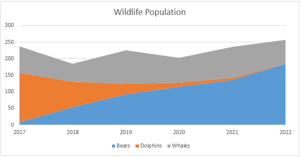
Area Chart in Excel - Easy Excel Tutorial

Visualizing Search Terms on Travel Sites - Excel Bubble Chart
Post a Comment for "42 excel graph data labels different series"